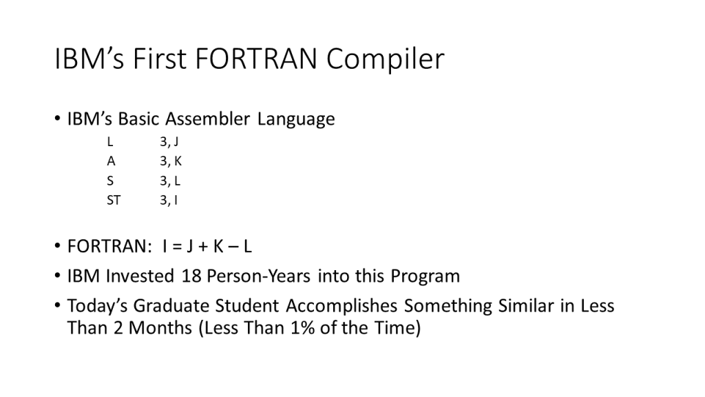
There is a story that illustrates the relationship between product size and the time that it take to develop it. In the truly early days of computers, they were programmed using Basic Assembly Language (BAL). If you wanted to add a couple of numbers in assembly language, you usually loaded one into a register and then added a memory location to that register. The code fragment above shows how the value of J + K – L might be assigned to I. It was tedious programming, but better than solving problems by hand.
In the 1950s, IBM introduced the first FORTRAN compiler. It allowed an assignment to be preformed by coding a statement like I = J + K – L. John Backus headed the project that developed that compiler. It took about 18 person years to develop. I was about 5 years old at that time. I had nothing to do with computers back then.
About 25 years later, I was teaching compiler design at New York Institute of Technology. It was a graduate course that I taught over the summer. I assigned each student the task of writing an interpreter. An interpreter is similar to a compiler. The difference will be described below. The point is that John Backus’s crew took about 286 person-months (18 person-years) to deliver their compiler. My graduate students delivered in less than 2 months. They were not working on this full time. They completed their software in less than 1% of the time that IBM had spent. There are important lessons about productivity and estimating to learn from this.
First of all, it was common for instructors of compiler design courses to require their students to develop an interpreter, not a compiler. A FORTRAN compiler would take a statement like I=J+K-L and transform it into the object code like the one shown in the slide above. That object code would then be executed. The compiler must decide which register to use and when it was best to unload a register to storage. This is called register allocation. Likewise, the compiler must generate the actual object code. It must know when to use each type of machine language instruction. This is called code generation. Interpreters do not have to do this. They hold the values for each variable in a symbol table and perform the operations on them directly, without generating object code. Both compilers and interpreters require the understanding of computer language grammars, lexical scanners and symbol tables. Instructors found that having their students develop interpreters instead of compilers taught them most of what they needed to learn while freeing them from the tedious programming that would be involved in implementing the compiler. This lowered both the functional and technical size of the program. It lowered the consumer size of the program. This corresponds to he agile advice to do the simplest thing that works. There are other reasons, which will be described below, why John Backus’s team would probably not have benefited from this approach. However, even if my students had been required to develop a compiler, it might have made sense for them to develop the interpreter first. They would have gotten experience with the front end of the compiler. They could have demonstrated it to anyone that had an interest in it. These people could then drive future development based on their experience with the interpreter. This is the idea behind lean marketing and their mandate to develop the Minimum Viable Product (MVP).
There was another consideration. John Backus’s team must have done most, if not all, of their programming using BAL. Most of my graduate students were using Pascal. That was the standard educational computer language at the time. The same problem that required 3,200 lines of BAL could probably be written in 910 lines of Pascal. These numbers are based on work done by Capers Jones. There is no question that this contributed to the increased productivity of the graduate students. Some people would say that the graduate students could write the program 3.5 times as fast because of this factor alone. Others would say the graduate students would only be twice as fast since much of the work of program development does not involve coding. In any case, there is no question that this added to the productivity increase.
As was already stated, the functional and technical size of the program was the consumer size. It is like the square footage of a house. All things being equal, larger houses take longer to build than smaller ones. However, in both software development and house building, all things are not equal. The construction method impacts how large the job will be from a producer point of view. For software development, the producer size is a function of the consumer size and the development language. The same interpreter written in Pascal is considerably smaller than one written in BAL. This is the major reason that the graduate students were so productive. However, there are still more reasons.
The COCOMO II model is used to estimate the effort required for software development. Size is the main driver, but there are several factors that scale software size. One is Precedentedness. This is the extent to which this project is similar to ones that the organization has undertaken in the past. IBM’s first FORTRAN compiler was unprecedented. It was the first of its kind. It was breakthrough computer science. By the Eighties, compiler construction was well understood. It was now routine software engineering. There were standard text books. Schools like NYIT had a track record for training students to develop compilers. Precedentedness went from very low to very high with a corresponding decrease in required effort.
COCOMO II also has cost drivers that act as effort multipliers. The most significant ones measure the impact of personnel capabilities. It is not possible to compare the capabilities of IBM employees in 1950 to graduate students in 1980. However, one of the cost drivers is based on the use of software tools. In the 1950s, there were editors and debuggers available. These increased in quality by the 1980s. This also contributed to the increase in productivity.
The effort in person-months can be given by the equation RAD EFF PM = 4.46 * SIZE ^ E * Product of 21 Cost Drivers. E = .91 + .01 * Sum of 5 Scale Factors. The cost drivers and scale factors will be described in later posts. The SIZE is determined by the equation SIZE = Sum for each Language Level (Number of function points * Percentage of functionality implemented using languages at that level * 320 / Language Level) / 1000.
Language Level is a concept that was introduced by Capers Jones in the Eighties. He produced tables of about 500 programming languages and reported how many lines of code would be necessary to implement a function point. He essentially continued this work as late as 2017. It is best not to even think about lines of code. QSM refers to a metric like this as a gearing factor because in allows developers to develop more function points with less effort, similar to a bicycle rider using a higher gear. For this model, these language levels have been consolidated and adjusted to simplify effort estimation:
- Language Level 3 are for lower productivity languages. These include C, COBOL and FORTRAN.
- Language Level 4 are traditionally higher productivity languages. They are mostly the languages that we thought were high productivity 40 years ago. Examples of these are Pascal and PL/I.
- Language Level 5 are scripting and interpretive languages like JavaScript, Lisp and Shell Script.
- Language Level 6 contains some modern commonly used languages like C++, Go, Java, PHP , Python and C#.
- Language Level 7 are modern high productivity languages like Ruby. Simulation languages like Simula are also on this level.
- Language Level 8 are data base systems like DB2 and Oracle.
- Language Level 12 are for languages like Perl, Delphi, Objective C, Visual Basic and HTML. Statistical packages like SPSS also fall into this category. Perl actually varies in productivity. Earlier studies assigned it a language level of 15, while recent ones assigned it a level of 9. The same is true for HTML; studies have given it language levels between 2 and 22.
- Language Level 16 are modern higher productivity languages that are often especially productive in certain domains. For example, a language like MUMPS is productive in the medical community. Crystal Reports is a report writer.
- Language Level 50 is the home of very high productivity languages that are usually special purpose. For example, mathematical packages like Mathematica belong here. There are process modeling packages like BPM that are very productive in the domain that they were designed for. Certain application generators belong at this level. Spreadsheet packages like Excel are also in this level.
Many applications today are developed using a blend of computer languages. HTML may be used for screen handling, while JavaScript is used for processing data. They have different language levels. Therefore, the SIZE will need to be developed as a weighted average of the different languages. The weights will be based on the relative amount of functionality that each language is being used to implement. This usually requires some estimating. This is because each elementary process might possibly be using more than one language for implementation. The estimator must consider this when prorating the language levels.
The next thing to calculate is the calendar time that this application should require. The primary driver is the effort required. Calendar time is a function of the effort but it is not a continuous function. The equations for calendar time are different depending upon the size of the project. In this case, the project size is measured in person months of effort. The effort figure from above could have been used, but for consistency with the COCOMO suite, a quantity called PMnoSCED is used. PMnoSCED is the effort figure from above / the product of the last 5 cost drivers / 1.43. PMnoSCED is based solely on COCOMO, which uses only the first 16 cost drivers. The value of 1.43 is the extra effort that is required for rapid delivery. As far as the formula is concerned, it is the value of SCED. Once this value is determined, the calendar time is determined by one of these alternatives:
- If the project is small, based on the value of PMnoSCED being less than or equal to 16 staff months, then the number of calendar months, called RAD EFF M, is equal to 1.125 * SQRT(PMnoSCED) * product of the last 5 cost drivers. The last cost driver has a different value for schedule than for effort. In any case, this value will be of no surprise to traditional project managers. It was common wisdom to staff a project by using the square root. For example, a 9 staff month project would be performed by 3 people in 3 months. The truth is that small projects can often be planned by identifying tasks and assigning people to them. The project plan becomes the estimate.
- If the project is large, based on the value of PMnoSCED being greater than or equal to 64 staff months, then RAD EFF M is equal to 3.1 * PMnoSCED ^ (.28 + .002 * the sum of 5 scale factors) * product of the last 5 cost drivers. This is delivery time from COCOMO, post processed by the CORADMO cost drivers. This is not surprising; COCOMO was built with large projects in mind.
- If the project has a value of PMnoSCED between 16 and 64 staff months, then the number of months is based on a linear interpolation between the number of months between the delivery time for a 16 staff month project and a 64 staff month project. It is based on this value, because the result is still post processed by the CORADMO cost drivers. Without considering this post processing, a 16 staff month process will be completed in 4 calendar months. The delivery time for a 64 staff month project, a value that can be referred to as Mof64 is given by 2.75 * 64^ (.002 * sum of 5 scale factors). The delivery time for the project, RAD EFF M, is equal to 1.125 * ((M of 64 – 4) / 48 * PMnoSCED) + (4 – 16 * (Mof64 – 4) / 48)) * the product of the last 5 cost drivers.
The team size is simply RAD EFF PM / RAD EFF M.
Leave a Reply