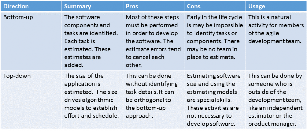
When most people think about estimating, they are thinking about bottom-up estimating. When your car needs to be repaired, you bring it to a mechanic. If you need new brakes, you will get an estimate for the cost of the brakes and the amount of time that is required to install them. If you also need an oil change, then the cost of that is added to your estimate. Software developers tend to think the same way. They attempt to identify the tasks that must be performed. They estimate the time for each task and add up these estimates. Agile developers do this. The steps of agile estimating are explained in Traditional Agile Estimating.
Some organizations already have Software Development Life Cycles (SDLCs) that they have specified. These SDLCs give all of the tasks that must be performed to develop software. However, many of the steps have to be broken down into finer detail. For example, there may be a task called Code Modules. However, that is both difficult to estimate or control. It ends up being broken into Code Payment Screen, Code A/R Report and a host of others. Early in the life cycle, it is very difficult to specify all of these tasks and impossible to estimate them.
People involved in agile development usually think of estimating from the bottom-up. They will identify as many user stories as possible early in the life cycle. They will then use a technique like estimating poker to assign story points. In summary, estimating poker is a collaborative technique that involves the development team. User stories are considered one at a time. Each team member assigns a number of story points to the story. They discuss it until they reach consensus and then move on to the next user story.
Managers love the idea of bottom-up estimating. If all of the tasks necessary to develop an application are estimated, they can be placed in a work breakdown structure and a Gantt chart. This gives the illusion of control. The developers love the idea of bottom-up estimating. Stories and tasks must be identified as part of the development process. Therefore, the bottom-up estimate is not extra work just associated with estimating. This is consistent with agile principles and practices. Statisticians love the idea of bottom up estimating. Whether estimating by task or user story, each component gets its own estimate. The estimates will usually be incorrect, but the errors will tend to cancel each other out. In theory, it is a winning approach. In practice, you just cannot do bottom-up estimating early in the life cycle. Project sponsors, end users and business analysts are developing any application artifacts like a feasibility study. Sponsors and users do not know what logical data models are. Business analysts know what they are, but probably have no idea how long it will take to develop one before the scope of the project is better established. For many applications, the development environment has not yet been decided on. Data warehouse applications may be developed using special software packages with entirely different development tasks than an organization typically specifies in its SDLC. In most cases, bottom-up estimating is impossible to do correctly early in the life cycle.
Top-down estimating begins with establishing the size of the application to be developed. Knowing this, algorithmic models were used to predict how much effort and how much calendar time would be required to develop the application. This approach was developed when the waterfall approach to software development was popular. Therefore, these models typically predicted how much time would be spent in the analysis, design and coding phases of the application development. Some approaches would predict the amount of time for various activities, like project management. In the beginning, that size was expressed in lines of code. There were two problems with this. First, you only know the number of lines of code after you have developed the application. Then you do not need the estimate. However, many organizations developed heuristics to help them predict lines of code. These rules of thumb were tied to the experience of the organization. For example, at one time NASA would predict the number of lines of code in satellite support software based on the weight of the satellite itself. The second problem can be summarized by Capers Jones’s statement the using lines of code should be considered professional malpractice. There are many problems with it. In one of his books, Capers shows that it often misrepresents the value of software. For example, is 2,000,000 lines of assembly language more valuable that 20,000 lines of COBOL?. Should it take 100 times longer to write? Even more to the point, with so many development environments being build around screen painters and other tools that do not actually have lines of code, the antiquated measure has become unusable. Function points, use case points and a host of lesser known measures have taken the place of lines of code. Barry Boehm (no relation) developed several estimating models that he called the Constructive Cost Model (COCOMO) in 1981. One of models was Basic COCOMO. It transformed the number of lines of code into the person-months of effort and the calendar months of schedule that would be required for application development. Practitioners at he time found ways to drive COCOMO from function points as opposed to lines of code.
Basic COCOMO was not as accurate as people wanted. Therefore, Boehm introduced Intermediate COCOMO at the same time. He actually introduced product level and component level versions of Intermediate COCOMO, but the difference is not important at this point. What is important is that Intermediate COCOMO utilized cost drivers. Cost drivers impacted the estimates. They were necessary and made sense. Imagine there are two applications that are 100,000 source lines of code. Will they take the same amount of time to develop? Probably not. There will be two types of differences between the two application projects. The first type are product differences. One application might be a computer game and the other an embedded system in a piece of medical equipment. The second application will have a higher required reliability. This will impact its development time. There are other product related cost drivers. The complexity of the products may also be different and impact the development time. The other class of cost drivers are associated with the development process. How experienced is the team with this type of application? How experienced is the team with the development language/environment being used? These cost drivers also impact development effort and schedule. In fact, cost drivers can change development effort by an order of magnitude.
COCOMO was not the only costing model around. At about this time, Larry Putnam introduced Software Lifecycle Management (SLIM). The Walston-Felix IBM-FSD Model and the Price-S model were two other top-down models that were introduced at about the same time. Which one was best? Nobody knows! There were several bake-offs but none actually answered that question. It turns out it was impossible to answer. Which car is best? In 1969, I saw a move called Grand Prix. Pete Aron is a race car driver who is just about unemployable. He was reckless. A Japanese car company hires him. He wins the race. Why? If you are reading this today, and obviously you are, then you might think it was because the Japanese are capable to making a fine automobile. In 1969, this would never of occurred to you. The Japanese had introduced motorcycle to America and they were a failure. Japanese cars would be the same. Pete Aron won the race because it is the driver, not the car that wins the race. He was driven to win and afraid to lose. That is all there was to it. Automotive enthusiasts might debate the. However, when it comes to estimating there is no debate. It is the estimator, not the model, that produces a useful estimate!
Practitioners started to use function points to drive the top-down models. Capers Jones had produced some tables that showed how many lines of code were required to implement a function point. Thus, function point could drive models like COCOMO. Some practitioners used unadjusted function points. There were complications when the Value Adjustment Factor (VAF) was used. Which General System Characteristics (GSCs) resulted in more lines of code? They were not adequate to use in place of cost drivers. A minimum VAF would make the adjusted function point size 65% of its unadjusted size; maximum would be 135%. The size difference is only a factor of 2. Cost drivers could usually impact the estimates to a much greater extent. Now, the International Function Point Users Group (IFPUG) has introduced the Software Non-functional Assessment Practices (SNAP). This is a counting approach that might replace the product cost drivers, but not the process ones.
These top-down techniques can often be performed by someone who is not familiar with all of the nuances of system development. The individuals must be familiar with the model being used, such as COCOMO. In addition, they must be trained in the sizing measure being used, such as function point analysis. This means that there is usually a small group of estimators in most organizations. In an organization using agile development, this might be a function that the product managers take on. This way, they can report back to the sponsors and other users what they expect in terms of schedule for an application development. Many organizations rely on consultants to perform these estimates. An independent estimator is often a good choice. This estimator is not overstating an estimate in order to negotiate for more resources, nor understating the estimate in order to pressure the development team to deliver faster.
Estimators look for techniques that are orthogonal to one another. This means that they are statistically independent. Top-down and bottom-up estimating approaches can be orthogonal. The bottom-up method is usually performed during the development just by virtue of identifying tasks and assigning people to them. If a top-down estimate has been developed, then it can be compared to what is being indicated by the bottom-up estimate at any time.
In the perfect world of agile systems development, all of the activity goes directly into developing application code. This is a drawback of top-down estimating. The effort that goes into it does not directly implement the application. If that effort is performed by a non-developer, then it becomes more of a business decision of whether the time and effort spent in developing the effort is helping the project sponsor to make better business decisions. Another area of concern is the distraction that this may be for the development and user communities. If the developers must answer questions in order to size the application, then this detracts from development effort. If a user must answer questions, then that user may be distressed if and when a developer asks the same questions again. The value of the estimate must exceed these costs or it should not be done.
The most modern of the cost models do not fit neatly into the bottom-up or top-down category. COCOMO II has replaced COCOMO the model of choice among COCOMO fans. SPQR, Checkpoint and Knowledge plan were released by Software Productivity Research (SPR), then under the direction of Capers Jones. Dan Galorath’s SEER-SEM is one of the more recent, commercially successful estimating models. The pros and cons of these approaches are basically the same as top-down models.
Leave a Reply